The R1D input defines the physical properties and discretization of the local subsystems. These are one-dimensional units which may be attached to any global block within the system. They may be used to simulate the second porosity of a fractured media or they may be used to broaden the boundaries of the global system at minimal expense. This particular capability of the SWIFT II code is described by Reeves et al. [1986a], Sections 2.3, 5.6 and 7.1.3.
If KSLVD = 0 (READ M-3), then all R1D input should be skipped.
4.1 PHYSICAL AND DISCRETIZATION PARAMETERS
READ R1D-1 (E10.0) Rock Compressibility.
A set of three records is read for each local rock type assuming a natural ordering of the rock types, i.e., IR = 1,2,..., NRTD.
DMFD1 Coefficient of thermal increase in diffusivity,
EF-1 (EC-1).
PHID Porosity.
AKSD Permeability, ft/d (m/s).
ALPD Dispersivity, ft (m).
UKTD Thermal conductivity, Btu/ft-d-EF (J/m-s-EC).
CPRKD Heat capacity, Btu/ft3-EF
(J/m3-EC).
1 - Prismatic structural units.
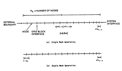
1 - Single-mesh generation.
2 - Double-mesh generation.
SAD, DSD and DSDO are used to generate nodal positions. See Figure 4-1b.
Reference: Reeves et al. [1986a], Section 7.1.3.
If KGRD 0 skip the following list.
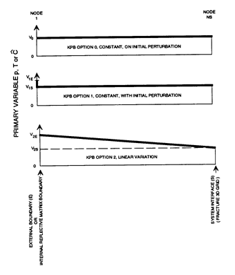
In this section boundary conditions for the outer extremity of the local subsystem and initial conditions for the local subsystem are prescribed for the primary variables as a function of local rock type. The boundary condition at the local/global interface is not under user control since it is always matched implicitly to the value of the corresponding global variable.
Enter as many records as necessary to define all initial and boundary conditions. Terminate the input here with a blank record. Even if no boundary specifications are desired, a blank record must still be used.
READ R1D-3 (LIST 1: 5I5; LIST 2: 3E10.0)
KBC Boundary-condition control
1 - Dirichlet conditions are taken for all primary variables.
2 - Dirichlet conditions are used for the variables T´ and a no-flux condition is used for P´ and C´.
3 - Dirichlet conditions are used for
the variables C´ and a no-flux condition is used for T´. Note:
A fluid flux is calculated due to density changes.
1 - The boundary condition is set at the value prescribed in List 2, and the initial condition is fixed at the global-block value.
2 - The boundary condition is set at the value prescribed in List 2, and the initial condition is fixed at the boundary-condition value.
3 - The boundary condition is set at
the value prescribed in List 2, and the initial condition varies directly
from the Dirichlet condition at the outer extremity to the global-block
value at the system interface.
KSWB Brine control. Operative for KBC
= 1 and KBC = 3 only. The options here are the same as that of KPB (see
Figure 4-2).
TPBD Specified boundary value for temperature, EF (EC).
SWBD Specified boundary value for brine
concentration, mass fraction.
Figure 4-2. Initial/boundary conditions for the primary
variables within the local subsystems.
4.3 DISTRIBUTION COEFFICIENTS
If there are no radioactive components, i.e., NCP = 0 (READ M-3), skip this input set. Otherwise read one data set for each rock type.
READ R1D-4 (7E10.0)
4.4 RADIONUCLIDE BOUNDARY CONDITIONS
Radionuclide boundary conditions are not under the direct control of the analyst. They are set internally to be consistent with the condition used for the flow. Thus, for a constant-pressure condition, a convective flux condition is set on the radionuclide transport. For a no-flow condition, of course, a no-flux condition is used for the radionuclide equation.
4.5 DUAL POROSITY BLOCK MODIFICATIONS
Follow the data listed below
with a blank record. If no modifications, a blank record is still required.
READ R1D-5 (LIST 1; 6I5; LIST 2: E10.0)
J1, J2 (Similar definition for the J index.)
K1, K2 (Similar definition
for the K index.)