In this chapter, special topics on input variables for SWIFT are discussed. For example, the definitions of permeability and compressibility are not always familiar to many hydrogeologists. These and other topics are briefly discussed to aid users in addressing the overlapping jargon of hydrogeologists and reservoir engineers.

Using nomenclature from the SWIFT model, the capacity of a geologic formation results from the compressibility of water, c_w, and the rock compressibility, c_r or total compressibility, c_t. These parameters may be combined with the formation porosity, f; water density, r; formation thickness, b; and the gravitational constant, g/g_c to form the storativity, S as follows:

 where the English units are:

Hydrogeologists typically define storativity in terms of the fluid compressibility, b, and the compressibility of the porous media, a, as follows:

in which terms are related by

         a = f C_r

        b = C_w

Exceptions to the above include J. Bear (1992) and DeWiest (1966). Note the differences and avoid confusing conventions.

Thus, if you know the storativity for an application and assume a value for water compressibility, the compressibility of rock can be calculated as:

         C_r = (144 S/b - rfC_w )/rf

12.2 CONVERSION OF PERMEABILITY UNITS

The SWIFT-2002 model requires input in the form of hydraulic conductivity. The code uses the reference condition (viscosity, and fluid density) and internally stores the permeability. It is convenient to convert formation permeability to hydraulic conductivity based on standard conditions of fresh water at ground surface conditions (fluid density equal to 62.4 lb/ft³). The conversion factor used is:

2.7 ft/day per d

Under variable density conditions one needs to include the effects of fluid density and viscosity. A more appropriate conversion is:

where

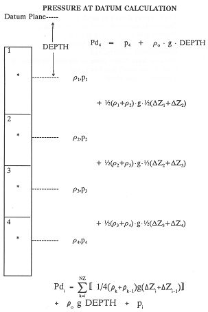
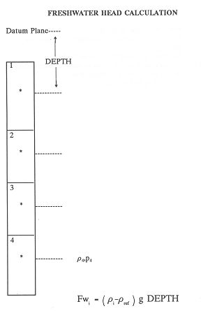
12.3 DEVELOPMENT OF PRESSURE AT DATUM

The SWIFT-2002 code uses the dependent variable pressure-at-elevation, or fluid pressure to calculate the groundwater flow under variable fluid density conditions. Intercell fluxes between adjacent finite-difference grid blocks are evaluated using the equations for the continuity of mass and Darcy's law for groundwater flow. The resulting partial differential equation is second order in space, wherein the intercell flow is defined by the harmonic mean to describe the flow transmissibility. This definition preserves mass flux and weights the intercell flows with the appropriate fluid density as well as the grid block dimensions, permeability and fluid viscosity.

Between two grid blocks, ground water flow is evaluated using the difference in the pressure at elevation (i.e., the difference in fluid pressure) and the difference in the block centroid elevation (i.e., the difference in elevation potential). Simply stated, the code evaluates the total potential difference, as composed of the fluid pressure and elevation potential.

The pressure at datum is a scheme to represent the equivalent total potential and can be defined in several ways. The datum plane is defined at a reference elevation, often taken as the ground surface or the top of the aquifer model. Pressure at elevation in each grid block is converted to a common basis, the datum plane, in order to create a display (i.e., isopleths of pressure or potentiometric surfaces) the potential field. The definition of pressure correction depends on the interpretation of the potential integral:

Reference: (Freeze and Cherry, 1979, equation 2.9, page 20)

where:

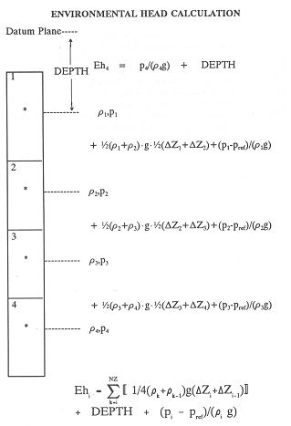
The first term is the elevation potential and the second is the fluid pressure recognizing that there is work involved in raising the fluid pressure from p = p_o to p = p. In the SWIFT-2002 model, the integral is defined by examining the columns of blocks and performing the integral as a summation using the block under consideration and all of the overlying grid blocks.

The following figures detail these methods of calculating the pressure.

12.4 MASS FRACTION VS DENSITY VS SPECIFIC GRAVITY

The relation between mass fraction vs fluid density vs specific gravity if often misunderstood. The relationship between specific gravity and fluid density is linear. Mass fraction used in SWIFT is almost, but not quite linear. Thus care should be taken in examining the results from simulations using SWIFT.
 

The definition of mass fraction is:

             mass of brine divided by mass of water

where: 

"water" is a fluid with the density defined by "BWRN".

"brine" is a fluid with the density defined by "BWRI".

The SWIFT model solves for conservation of mass and the fluid density is allowed to vary linearly. The density is a linear function of pressure (compressibility of water), temperature (coefficient of thermal expansion) and chemical composition (as defined by the two fluid densities BWRN and BWRI). 

On the next page is an example set of calculations, based on the above definition. Note that the middle specific gravity 1.08 = 1/2 (1.00 +1.16), the scaled mass fraction is 0.537, not 0.500.
 
 

The definition of grid block saturation is defined as:

_{where Po if the reference pressure PINIT R1-16.}  

_{Take the example where Po is zero.  For a block to be fully saturated, the pressure would be positive.  When the pressure at elevation (fluid pressure) is zero, the block id 50% saturated.}